Zero-Knowledge Proof - Cryptographic Primitives and Sigma Protocol
This blog covers the use of mathematics and cryptography in zero-knowledge protocols, specifically discussing elliptic curves, Pedersen commitments, and the Sigma protocol. It provides an overview of these concepts and their relevance in blockchain.
ByVitali Bestolkau — Explainers
15 min read
Introduction
This article is an overview of mathematics and cryptography as they relate to zero-knowledge protocols. Our goal is to provide a simplified introduction to these concepts, focusing on the math and cryptography principles used in the Sigma protocol. It's important to note that the Sigma protocol is just one example of a zero-knowledge protocol. It is not necessarily representative of other protocols such as ZK-SNARKS, ZK-STARKS, or Bulletproofs. However, the Sigma protocol implements many cryptographic primitives widely used in the field and has also found applications in the blockchain industry. This article aims to provide a general understanding of these concepts and their significance in Zero-Knowledge protocols.
1 Elliptic Curve
1.1 What is it
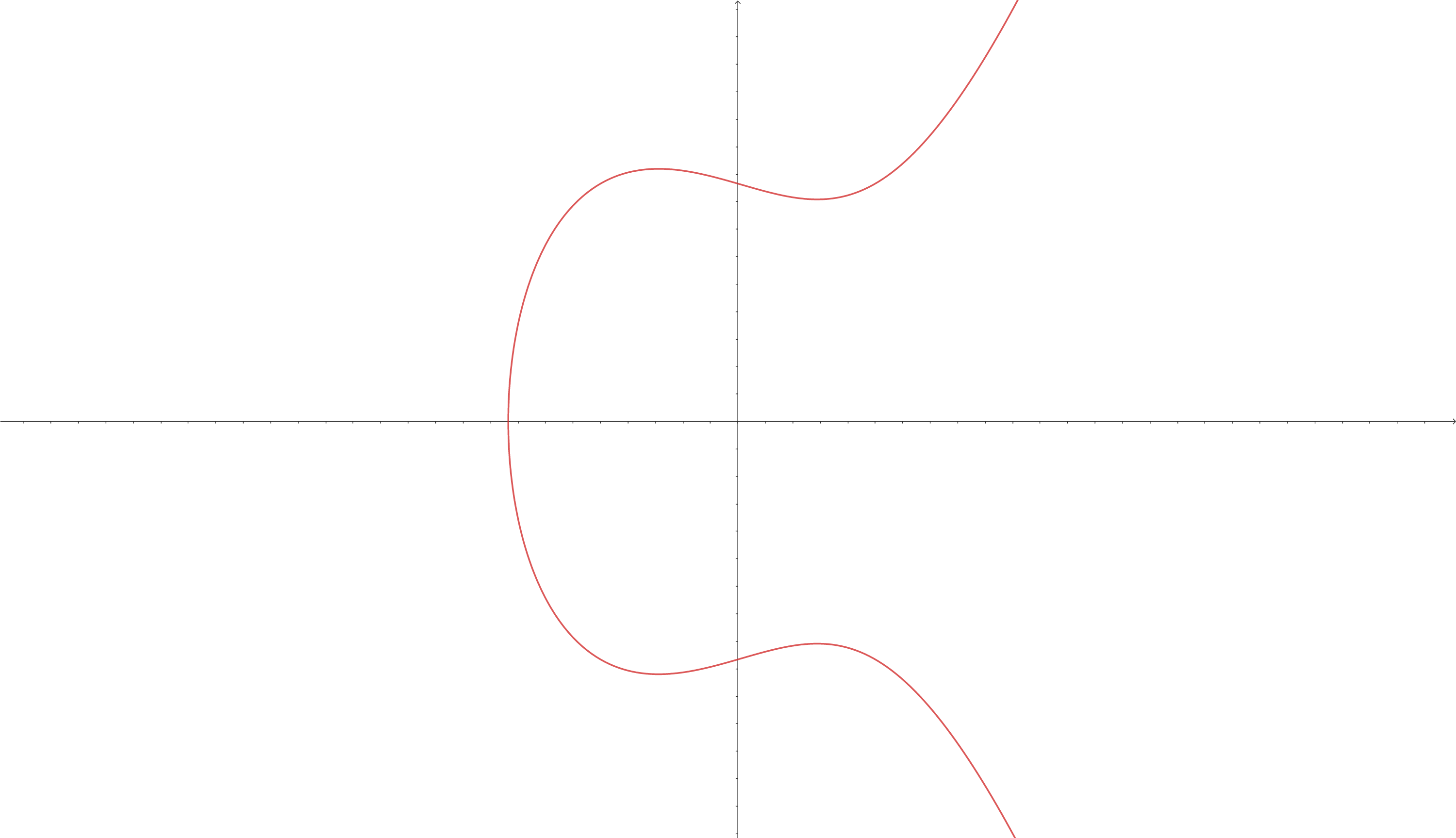
Elliptic Curves (ECs) are cryptographic primitives that are widely used in modern cryptography. They are defined by the equation and have a specific shape. ECs are used in public-key encryption and the Elliptic Curve Digital Signature Algorithm (ECDSA), which was previously used for creating signatures in the Bitcoin blockchain for transaction verification. ECs are powerful tools that allow for the performance of various mathematical operations in cryptography.
In general, an Elliptic Curve looks like this:
💡
Note: Not all Elliptic Curves look this way. The way they look depends on the constants and . In the example, and , which makes the final equation looks like this:
To make the set of points on an elliptic curve finite, the values of and are capped at a large prime number , so that . This can also be expressed as .
1.2 How does it help to encrypt and decrypt data securely?
Elliptic curves can be used to securely encrypt and decrypt data through the use of public and private keys. Both sides (sender and receiver) must first "agree" on the specific EC to be used, including its constants and and the maximum value of the prime number . They also choose a random point on this EC, which they will use.
The sender and receiver then use their private keys, and , respectively, to calculate their respective public keys. Public key generation is done through the following equations: and , where and are new points on the EC and the public keys.
💡
Note: the Elliptic Curve Math differs from common Math. Check the source if you want to learn more about how multiplication and other operations work. Or you can check this video for the explanation of point addition.
To send the information, the sender:
- Encrypts the data using the receiver's public key .
- Sends the encrypted data to the receiver.
- The receiver decrypts the data using their private key .
If the receiver wants to reply to the received information, they can follow the same process but use the sender's public key instead of . When the sender receives the data, they can decrypt it using their private key .
The EC public key encryption scheme is considered secure because the private key computation involves the "elliptic curve discrete logarithm function," which is infeasible to compute for modern (non-quantum) computers (check the source for more). Thanks to the discrete logarithm problem, both public keys, and , can be made public along with the initial EC point . If an individual knows both and from the equation , it is almost impossible for them to compute the private key due to the difficulty of the discrete logarithm problem.
2 Pedersen Commitment
2.1 What is a commitment for
Commitments (or commitment schemes) are cryptographic primitives that securely send data that can only be verified when the sender (prover) reveals the data. Once the data is disclosed, the verifier calculates a new commitment using the revealed values and compares it to the original commitment sent by the prover.
2.2 Commitment properties
Commitments have two crucial properties: binding and hiding.
- Binding: means that the value included in the commitment is fixed (defined) and cannot be altered after the commitment is created.
- Hiding: means that the value included in the commitment is hidden and cannot be viewed by anyone until it is "officially" revealed.
2.3 Reasons for Pedersen Commitment
While elliptic curves (ECs) can be used for secure data transfer by encrypting a hidden value, typically, this value is within a small range (e.g., from 1 to 10), which makes it vulnerable to brute force attacks. That's where Pedersen commitments come in.
2.4 Pedersen Commitment Details
Pedersen Commitments address this issue by introducing a "blinding factor," a randomly generated number from a large range , which is used to "blind" the committed value. This blinding factor helps to obscure the committed value, making it more difficult for an attacker to guess the value through brute force methods.
But can not be added to the committed value and have , where is a point on an elliptic curve. That would violate the binding property. After making a commitment, the committer may reveal not values and , but instead values and , where and , and they would still provide the right outcome.
In Pedersen Commitments, in addition to , we have another point on an elliptic curve. Then we get the following commitment formula: . Although, most commonly, a Pedersen Commitment is represented like:
Where are public generators of a cyclic group of prime order . is also called the opening of the commitment.
💡
is a function. But why do we provide (only) two variables? Because everything except and is public. and are the only unknown variables before the function is executed.
💡
Different articles show different mathematical approaches in the same context.
Some articles use the Elliptic Curve Math to explain Pedersen commitments and the Sigma protocol (which is presented further in the article), which in the case of the commitments, would look like , where and are points on an EC.
Other articles use logarithms to show the math behind these principles. The Pedersen commitment case would look the same as shown earlier in the article: .
In the context of this article, these versions can be considered equal because they are both based on the discrete logarithm problem. But this article will stick to the logarithm version from now on.
2.5 How Pedersen Commitments work
In a nutshell, Pedersen Commitments work the following way:
A prover is a person/party trying to prove the validity of the data they provide. A verifier is a person/party that verifies the validity of the received data.
- The prover selects a secret value .
- A random number (as a blinding factor) is generated.
- The prover creates a commitment using the previous two values: and sends it to the verifier.
- The prover reveals values and .
- The verifier calculates with the revealed values: and checks if .
💡
It is worth mentioning that the Pedersen commitments are not Zero Knowledge, as they rely on the private data being revealed in the end.
3 Sigma protocols
❗
This section is mostly based on this article that perfectly explains on a high level how the Sigma protocol works.
Sigma protocols are Proof of Knowledge (or, in this context, an interactive Zero-Knowledge Proof (ZKP), more about that here) protocols that consist of three phases:
- Commitment phase. The prover decides on the value they are trying to prove, creates a commitment out of this, and sends the commitment to the verifier.
- Challenge phase. The verifier comes up with a challenge and sends it to the prover.
- Response phase. The prover generates a response and sends it to the verifier.
The verifier can then determine if the prover knows the value based on the response received.
💡
Even though the Sigma protocol is Zero-Knowledge, it is not connected to the ZK-SNARKs, ZK-STARKs, or Bulletproofs, as those protocols work differently from the Sigma protocol. However, they may share some similarities.
💡
The Sigma protocols are ZKP, but one of their main disadvantages is that they rely on the fact that the verifier is honest. In the case of a dishonest verifier, the protocol will fail. At the same time, zk-SNARKs, Bulletproofs, and zk-STARKs do not have this issue.
Note: there can be a more detailed comparison of advantages and disadvantages between the Sigma protocol and other ZKP protocols, but the scope of this article will limit itself to only this disadvantage.
3.1 Schnorr Protocol
The Schnorr protocol is one of the most used Proofs of Knowledge. It is also a variation of a Sigma protocol, as it follows the three-step structure. It involves a prover attempting to prove to a verifier that they know the value of , where is a generator of a cyclic group of order , is public, and is private and known only to the prover.
💡
Note: Usually, in the context of Zero Knowledge, the private value that is being verified is called witness (in this case, is the witness). This article uses this word sometimes as well.
Check one of our previous articles to get a better insight into the Zero-Knowledge context
- The prover generates a random number and calculates a commitment . The commitment is then sent to the verifier.
- The verifier generates a challenge and sends it to the prover.
- The prover calculates and sends to the verifier.
The verifier checks if the equation is correct. If it is, then it is considered that the prover knows the witness (secret value) .
💡
Why does the verifier check the equation to prove the prover's knowledge of ?
Firstly, this equation consists only of public values and does not reveal the private ones: or .
Secondly, this equation must be equal in the end. That is because: , but as the initial statement says, , which means that and from the step 1 in the protocol it is said that , so in the end, we will get . Therefore, if the prover takes all the steps correctly, the final equation should be correct.
Thirdly, the third step kills two birds with one stone.
The prover hides their private value , as the verifier can not calculate the without knowing .
The verifier is assured that the prover does not cheat because it is only possible to calculate the response in advance for the final check passed by knowing either the random value or the challenge .
3.2 Fiat-Shamir Heuristic
The previous example is interactive, making a prover and a verifier communicate and stay online until the end of the process. The Fiat-Shamir Heuristic is a technique that converts interactive Zero-Knowledge Proofs into non-interactive ZKPs, which can also be used as a digital signature.
3.2.1 How it works
The prover needs to prove the knowledge of in , which is the same as .
- Prover generates a random number and calculates the commitment .
- Instead of receiving a challenge from the verifier, the prover calculates it by hashing into : .
- The prover calculates the response and sends a tuple to the verifier.
- The verifier calculates and checks if the equation is correct.
Alternatively, the prover can send the challenge to the verifier, who then calculates their own challenge and compares it to the one received from the prover. The process is as follows:
Same as earlier, the prover is trying to prove the knowledge of in .
- The prover generates a random number and calculates the commitment .
- The prover calculates the challenge .
- The prover calculates the response and sends a tuple to the verifier. (instead of , as the prover did in the previous example)
Now the verifier does the following:
- Instead of checking equality in the equation , they get a formula for the commitment , which will be and calculates this .
- Then the verifier calculates and checks if the calculated challenge is equal to the previously provided one: .
3.3 Schnorr signatures
In general terms, a (digital) signature is proof that the owner of a particular public key signed some data. The signature lets everyone confirm that the person with the public key signed some data using their private key without revealing the signer's private key to others. (Check the source for more)
Schnorr signature is used in validating transactions on the Bitcoin blockchain. To be more specific, it tells everyone that the sender is the one who owns the coins which are being transferred.
For their verification, Shnorr signatures use the Shnorr protocol, which implements the second version of the Fiat-Shamir Heuristic. However, while calculating the challenge , a new public variable is added. This variable is usually called message , which is a transaction itself (meaning the transaction's hash). So, the verification of in , knowing the message , looks the following way:
- The prover generates a random value and calculates a commitment .
- The prover calculates a challenge .
- The prover calculates the response and sends a tuple to the verifier.
- The verifier calculates the commitment , finds the challenge , and checks if . If the challenges are equal, the signature is considered valid.
3.4 Sigma protocol for Pedersen Commitment
Sigma protocol adds a Zero Knowledge layer to the Pedersen Commitments usage, as the private values are initially revealed in the end.
3.4.1 Knowledge of the opening in Pedersen commitment
The prover wants to verify that they know the value and the random number from .
- The prover generates random values and and calculates a commitment .
- The prover calculates the challenge .
- The prover creates two responses and . And sends to the verifier.
- The verifier checks if the equation is correct.
💡
Note: for these examples, the number of random values that should be generated in the first step of every Sigma protocol is equal to the number of private variables. The private variables that should not be revealed to the verifier but still should be proved to be known (in the case of Pedersen commitment, the private variable is a value together with a random number in ). As in the third step, the prover creates the same number of responses.
💡
If you want more examples of the Sigma protocol usage, check this source.
4 Recollection
💡
Elliptic Curves (EC) are one of the most well-known cryptographic primitives used in public-key encryption, blockchain, and Zero-Knowledge Proof. ECs are secure for large numbers, as the private key computation, also called the "elliptic curve discrete logarithm function," is infeasible for modern (non-quantum) computers.
💡
Pedersen commitments are used to transfer data that is in a small range securely, and that can be brute-forced. Pedersen commitments use Elliptic Curve Cryptography (ECC) as their basis, but they also add a Blinding factor, making the transferred data infeasible to learn.
💡
Pedersen commitments (like other commitments) have two main properties:
- Binding — the submitted values are defined and can not be altered after the commitment is created.
- Hiding — the submitted data stays hidden until the prover reveals it.
💡
Sigma protocol is an interactive Zero-Knowledge protocol that has three main steps/phases:
- Commitment phase. The prover creates a commitment and sends it to the verifier.
- Challenge phase. The verifier creates a challenge and sends it to the prover.
- Response phase. The prover calculates a response to the challenge and sends it to the verifier.
In the end verifier checks if the response is correct and tells the prover they are (the verifier) convinced.
💡
Sigma protocol has similarities with more well-known protocols: zk-SNARKs, Bulletproofs, and zk-STARKs, but they are not the same, and the mathematics used in those protocols is more advanced than for the Sigma protocols.
Moreover, compared to others, one of the main disadvantages of the Sigma protocol is that it relies on an honest verifier.
💡
Fiat-Shamir Heuristic helps make a Sigma protocol non-interactive and usable for applications.
💡
Schnorr protocol is one of the most used Sigma protocols.
💡
Shnorr signatures work based on non-interactive Schnorr protocols but add another public value to the equation, usually called message . In the context of blockchain, the message is a hash of the transaction where the signature is used.
5 Conclusion
This article provided an overview of several cryptographic primitives commonly used in Zero-Knowledge Proofs, including elliptic curve cryptography and Pedersen commitments. The article also described the structure and mechanics of Sigma protocols and demonstrated how they could be used to verify various data types, including Schnorr signatures. The following article will present a basic Proof of Concept for implementing Zero-Knowledge protocols.
More Resources
Elliptic Curve
- Elliptic Curves - Computerphile
- A Primer on Elliptic Curve Cryptography
- Elliptic curve point multiplication
- How Elliptic Curve Cryptography Works
- Elliptic Curve Cryptography: A Basic Introduction
- Elliptic Curve Cryptography (ECC)